Other posts in series
Introduction
I have started a new project. I had another look at the Kaggle datasets and chose this Santander dataset. The data is (superficially?) similar to that from the Credit Card Fraud dataset I have previously analysed: the data is clean, all numerical, and the task is to create a binary classifier. A big difference is that this Santander dataset has 200 features, whereas the Credit Card Fraud one had only 30 features. I presume this will make a difference (maybe I have to do some feature selection?), but I guess I will find out soon! Another difference is that we have two datasets: a training dataset on which we should create our models, and a testing dataset on which we use our models to make predictions which are then submitted to Kaggle.
Like with the credit card fraud project, I will start this one by creating some default models, and hopefully gain some ideas on how I ought to progress.
Default models
Some minimal data exploration shows that 90% of the training data has a target feature of 0 and 10% has target feature of 1. Due to this skew, I decide to us AUPRC to evaluate the models. Note that I split this training set further into a sub-training set and sub-testing set, fit the models on the sub-training set and evaluate the models using AUPRC on the sub-testing test. (Is there better terminology for this kind of thing?!).
Also, I did minor pre-processing, namely, I re-scaled the features to have a mean of 0 and a standard deviation of 1.
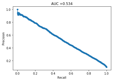
Logistic Regression
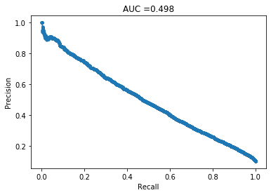 This does not look good. Lets see how other models do.
Decision Tree
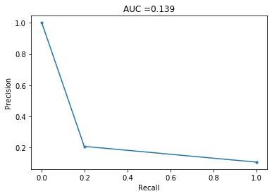 This does even worse! I guess this should be expected of decision trees. It is also worth noting that this took a couple of minutes to create, so I decided not to create a random forest, because I presume it would take a very long time.
kNN
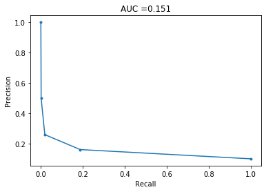 This also does poorly. However, I recently started reading Elements of Statistical Learning and it describes the ‘curse of dimensionality’, so I am not surprised by this low performance. Roughly, if you have many features, the nearest neighbours of a point are unlikely to be close to the point, and so not representative of that point.
XGboost
 This has basically the same PRC as logistic regression, and much worse than what was achieved in the default credit card dataset.
SVM
 And once again, a similar PRC to logistic regression and xgboost. Note that this one took a few hours to complete, so I will not be using these again for this project.
Handmade model
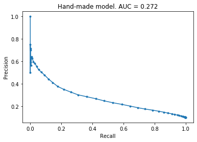 I used the same handmade model that I created in the credit card fraud project over here. As can be seen, this performance is in between the worst so far (decision tree and knn) and the best so far (xgboost, regression, svm). To me, this suggests that main issue is not with the number of features, but that maybe the dataset itself is difficult to work with and that it is hard to distinguish between the two classes.
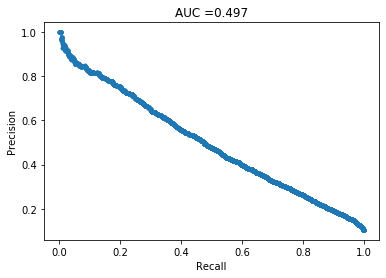
Random model
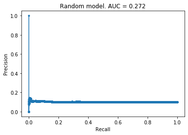 Based on all these graphs above, it was clear I had misunderstood something basic about the PRC graph. I believed that the worst case scenario for this curve was a straight line joining the two corners, and initially thought that these models were doing either worse or just as good as a random model. After thinking for a bit, I realised my mis-understanding. To confirm my feelings, I created a purely random model and the PRC is above. This curve makes sense: we get a straight line with a precision of 0.1 because 10% of the data has a target value of 1. If you’re just making random guesses, then you should expect that 10% of the predicted positive cases are truly positive, i.e., you should expect to get a precision of 0.1.
I think this misunderstanding arose because I got mixed up with ROC curves, in which a random model does produce a straight line.
Next steps
I will try to improve the models by doing some feature selection.