Visualising L1 and L2 regularisation

Introduction

In this medium post comparing L1 and L2 regularisation there is an image showing how L1 regularisation is more likely to make one of the parameters equal to zero than L2 regularisation.

One of my co-fellows at Faculty pointed out that this image is not convincing, because it could just be a case of a cherry-picked cost function. As I had never made any effort to properly understand L1 versus L2 regularisation previously, this was good motivation for me to better to understand.

The results are bunch of visuals that are below.

Varying cost function with parameters restricted to L1 or L2 balls

Parameters restricted to L1 ball

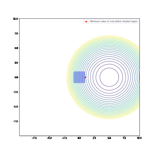
Parameters restricted to L2 ball

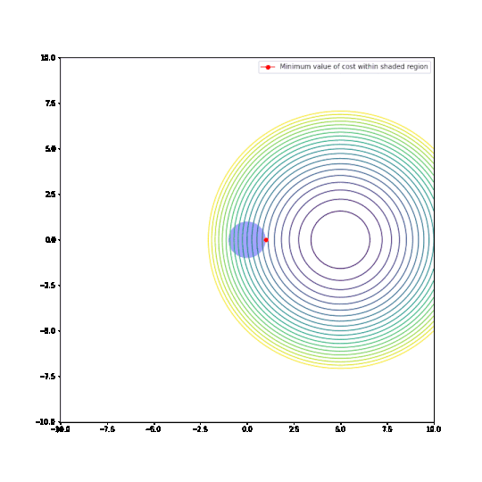
In the plots above:

The circular things that are moving around are contour plots of cost functions. They are all convex.
The shaded regions are L1 and L2 balls, i.e. all points where the L1 or L2 norm of the parameters are less than some fixed radius r.
The red dot is the parameter which minimizes the cost function, given the restriction of being within the ballh.

What can be seen is that restricting the parameters to an L1-ball results in one of the two paramaters being zero, most of the time. The L2-ball has no preference for values.

This matches the general descriptions I have seen of L1 regularisation in various blog posts and articles.

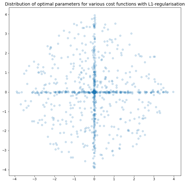
Varying cost functions with L1 or L2 regularisations

An issue with the above plots is that I have forced my parameters to be within an L1 or L2 ball. In regularisation, the parameters can have any value, but there is a regularisation term added to incentivise the model to reduce the L1 or L2 norm.

(Having this forced restriction corresponds to having a regularisation term that is zero if the parameters are inside the ball and infinity if the parameters are outside the ball. So normal regularisation can be thought of as being a smoothed out version of this forced restriction.)

To check that the insights gained in the above plots do work when we have regularisation I created a couple more plots.

I created a cost function (x-x0)^2 + (y-y0))^2 + r*norm((x,y))
r is a regularisation constant.
norm is the L1 norm in the first plot and the L2 norm in the second plot.
I determined the coordinates (x', y') that minimised the cost function above.
I added those coordinates to a scatterplot.
I then varied x0 and y0, producing many cost functions, and plotting the resulting (x', y') coordinates in the scatterplot.

Optimal parameters with L1 regularisation

Optimal parameters with L2 regularisation

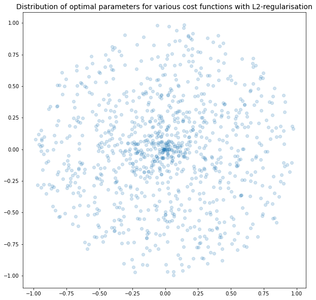
We can see in the plots above that the pattern continues. L1 regularisation will force parameters to zero, and L2 regularisation does not have any preferred direction - L2 just wants the length of the vector to be smaller.

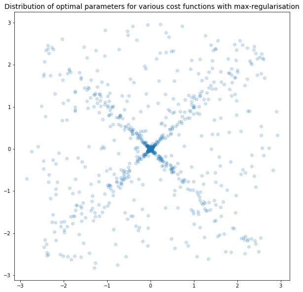
Max norm

To check your understanding, imagine how the plots above would look if we replaced the L1 and L2 norms with the max norm, max_norm((x,y)) = max(|x|, |y|).

No really, take a couple of minutes to think this through. You learn the most by actively engaging with the ideas rather than passively reading somebody else’s thoughts.

…

Well, here are the two plots. Minor note, the plots are for the L10 norm, but it is a good enough approximation to the max-norm.

Conclusions

I am glad I produced these plots. I have read before that L1-regularisation ought to have parameters go to zero, but I never really understood it, but now I have some feel for it. Also, it was good python practice.

Other posts in series