My thinking and plan

When doing the initial investigations, I noticed it took some time for the fitting, in particular for the random forest models to be fit. I want to do some hyper-parameter optimisations, but do not want to wait hours for it. Therefore, I wanted to reduce the time it takes.

I figured that 10% of the non-fraudulent data should contain most of the patterns that 100% of the non-fraudulent data does, and presumably having smaller datasets reduced the run time.

To reduce the datasets, I first split the data using train_test_split as normal. Then, I kept only those non-fraudulent entries whose index had final digit 0 - so I only have 10% remaining.

To better understand the effect removing data has, I tried removing different amounts of data, from 50% to 99%. The code for all this is at the bottom of the page.

Results for Random Forests

The charts below show what happened as I varied how much data was removed.

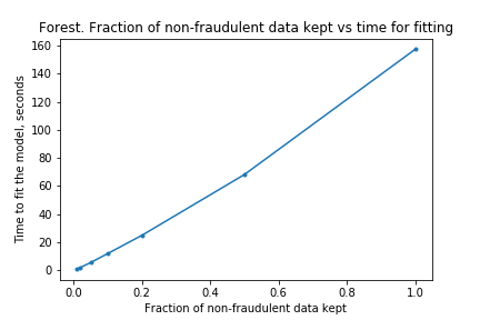
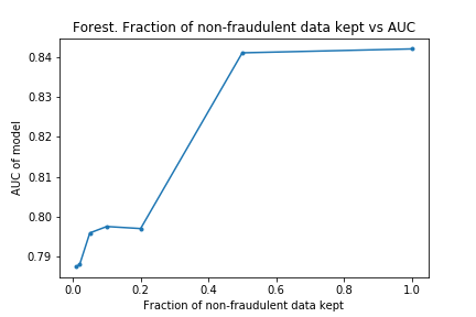
As I hoped, the time taken for the fitting to take place reduces as the dataset is made smaller. (In fact, time taken is linear with size of dataset. I don’t know if this is surprising or not, but I imagine it is clear if one knows implementation details of the algorithms). Also as I predicted, the effectiveness does not drop considerably by removing data.

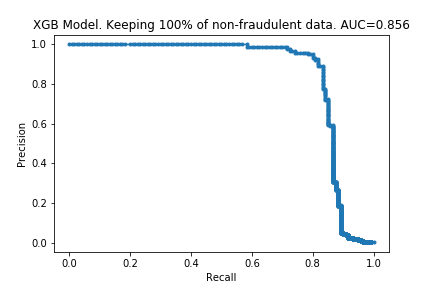
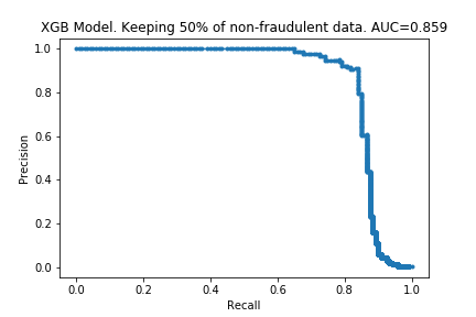
The charts below show some of the resulting AUC curves, so we can see where the drop in performance occurs.

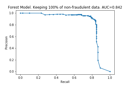
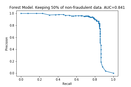
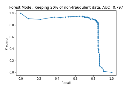
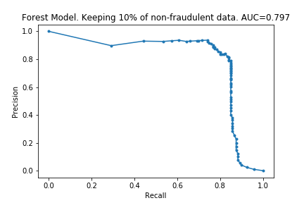
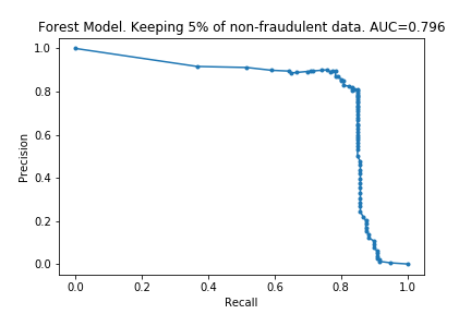
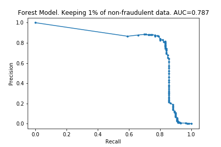
We can see that removing non-fraudulent data has resulted in reduced precision, with no visible drop in recall. This makes sense: I did not remove any of the fraudulent entries, so it looks like the models were still able extract the same information about them.

This is encouraging. In the context of credit card fraud, recall is more important than precision: the cost of fraud is greater than cost of annoying customers by mis-labelling their transactions as fraudulent.

Results for XGBoost

I ran the process on XGBoost models too. The charts are below.

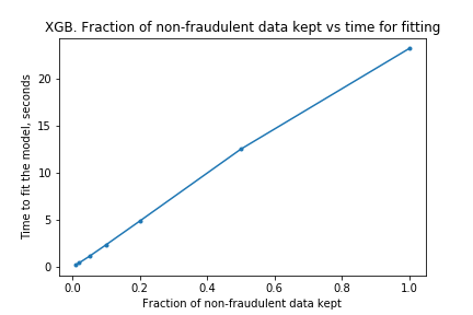
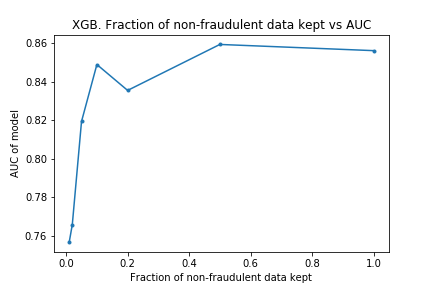
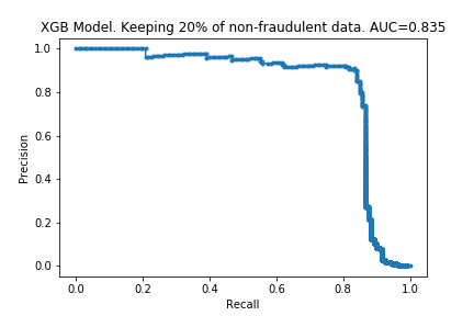
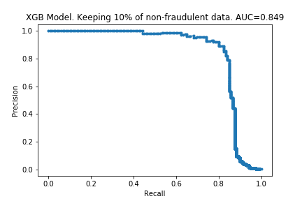
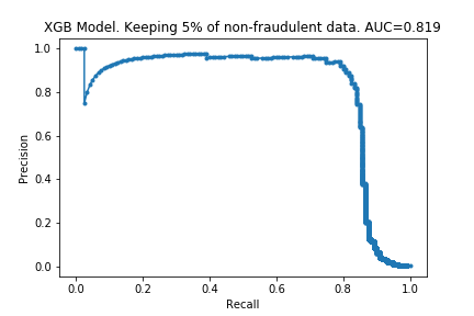
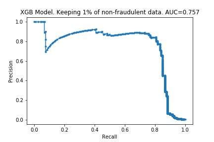
The results are similar to those for the random forest. The compute time is linear with the amount of data kept, and performance does not drop much either. Surprisingly, the performance is almost the same with only 10% of the data: only a 0.007 drop in the AUC! It looks like XGBoost is more ‘data-efficient’ than Random Forest: to get good performance, XGBoost requires less data than Random Forests.

Next steps

The next steps will be to do some hyper-parameter optimisations. But before that, like mentioned in Part 1, I want to better understand the data by creating a crude hand-made model. It will be interesting to see how it compares! My hope is to get an AUC of 0.7.

The code

Below is the code to produce the XGBoost models and charts. The code for Random Forest is similar.

# import modules
import numpy as np
import pandas as pd

from sklearn.model_selection import train_test_split
from sklearn.metrics import precision_recall_curve
from sklearn.metrics import auc

from matplotlib import pyplot as plt

from sklearn.ensemble import RandomForestClassifier
from xgboost import XGBClassifier

from datetime import datetime



# import data and create train_test split
data = pd.read_csv("creditcard.csv")
y = data.Class
X = data.drop(['Class'], axis = 1)
Xt, Xv, yt, yv = train_test_split(X,y, random_state=0)



# create function which takes model and data
# returns auc, time taken, and saves plot.

def auc_model(model, title, saveas, Xt, Xv, yt, yv):
    t0 = datetime.now()
    model.fit(Xt,yt)
    t1 = datetime.now()
    
    time = t1 - t0
    time = time.total_seconds()
    
    preds = model.predict_proba(Xv)
    preds = preds[:,1]
    
    precision, recall, _ = precision_recall_curve(yv, preds)
    auc_current = auc(recall, precision)
    
    plt.figure()
    plt.plot(recall, precision, marker='.', label='basic')
    plt.xlabel('Recall')
    plt.ylabel('Precision')
    plt.title(title + f'. AUC={auc_current:.3f}')
    plt.savefig(saveas + '.png')
    
    return time, auc_current



# create multiply xgb models with varying amount of data removed

model_xgb = XGBClassifier()

fraction_kept = [1,0.5,0.2,0.1,0.05,0.02,0.01]
times = []
aucs = []

for f in fraction_kept:
    selection = (Xt.index % (1/f) == 0) | (yt == 1)
    Xt_reduced = Xt[selection]
    yt_reduced = yt[selection]
    title = f'XGB Model. Keeping {100*f:.0f}% of non-fraudulent data'
    saveas = f'creditcard_2_xgb_{100*f:.0f}'
    
    time_new, auc_new = auc_model(model_xgb, title, saveas, Xt_reduced, Xv, yt_reduced, yv)
    times.append(time_new)
    aucs.append(auc_new)



# plot charts to show effect of changing fraction of non-frauduluent data removed
plt.figure()
plt.plot(fraction_kept, times, marker='.')
plt.xlabel('Fraction of non-fraudulent data kept')
plt.ylabel('Time to fit the model, seconds')
plt.title('XGB. Fraction of non-fraudulent data kept vs time for fitting')
plt.savefig('creditcard_2_xgb_times')

plt.figure()
plt.plot(fraction_kept, aucs, marker='.')
plt.xlabel('Fraction of non-fraudulent data kept')
plt.ylabel('AUC of model')
plt.title('XGB. Fraction of non-fraudulent data kept vs AUC')
plt.savefig('creditcard_2_xgb_aucs')

Investigating Credit Card Fraud, Part II, Removing data

Other posts in series

My thinking and plan

Results for Random Forests

Results for XGBoost

Next steps

The code