- Other posts in series
- Forest model, hyper-parameter selection
- Forest model, final model
- XGBoost model
- Next time
- The code
Other posts in series
Forest model, hyper-parameter selection
I tidied up the code from yesterday to allow me to optimise for more than one parameter at once. For each combination of hyper-parameters, I obtained 20 different AUCs (by using five 4-fold cross validations). The results were stored in a pandas dataframe. The code for this is at the bottom of the page.
I then averaged over all the folds and sorted the results. The code for this and the output is below.
auc_forest.max_depth.fillna(value = 0, inplace = True)
auc_forest_mean = auc_forest.groupby(['n_estimators', 'max_depth', 'max_features']).auc.mean()
auc_forest_mean.sort_values(ascending = False).head(20)

n_estimators  max_depth  max_features    auc
50.0          0.0        10.0            0.774015
              50.0       10.0            0.774015
60.0          0.0        10.0            0.772589
              50.0       10.0            0.772589
              10.0       10.0            0.772573
50.0          10.0       10.0            0.772328
40.0          10.0       10.0            0.771290
80.0          0.0        10.0            0.771108
              50.0       10.0            0.771108
40.0          0.0        10.0            0.770744
              50.0       10.0            0.770744
50.0          0.0        7.0             0.770522
              50.0       7.0             0.770522
80.0          10.0       10.0            0.770487
50.0          10.0       7.0             0.770472
60.0          50.0       7.0             0.770472
              0.0        7.0             0.770472
              10.0       7.0             0.770025
40.0          50.0       5.0             0.769278
                         auto            0.769278
A few things were found by doing this:
- The best options for the hyper-parameters are n_estimators = 50, max_depth = None and max_features = 10.
- max_depth = None and max_depth = 50 produced the same models. This means that maximum depth achieved without any limits is less than 50.
- max_features = auto and max_features = 5 produced the same models. This is obvious in retrospect: auto means taking the square root of the number of features, and we had about 30 features.
Forest model, final model
Using these hyper-parameters, I created a the final Random Forest model. The precision-recall curve is below:
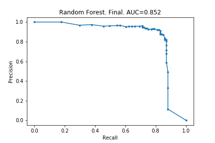
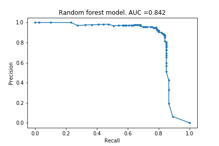
For comparison, the very first random forest model is also included. As can be seen, there is an improvement but a seemingly minimal one. Based on examples I have seen elsewhere, these minor improvements are what can be expected from hyper-parameter optimisations.
XGBoost model
I repeated the process above for XGBoost models. The best parameter settings were as follows:
n_estimators  max_depth  learning_rate    auc
50.0          5.0        0.05             0.761125
100.0         5.0        0.02             0.760002
50.0          10.0       0.05             0.759094
              15.0       0.05             0.758146
100.0         10.0       0.02             0.757185
              15.0       0.02             0.756748
200.0         10.0       0.02             0.747032
              15.0       0.02             0.743830
50.0          15.0       0.10             0.742954
              10.0       0.10             0.739922
100.0         10.0       0.05             0.737840
              15.0       0.05             0.737013
50.0          10.0       0.02             0.729299
              15.0       0.02             0.729239
              5.0        0.02             0.729049
200.0         5.0        0.02             0.727433
50.0          15.0       0.30             0.726696
              5.0        0.20             0.726479
100.0         5.0        0.20             0.724851
              15.0       0.30             0.722728
Using the settings from the top row, I created my final model, whose precision-recall curve is below. I have included the original curve, too.
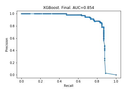
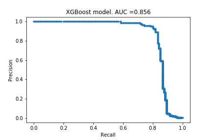
!! After doing the optimisations, the model became worse! The AUC decreased by 0.002. The explanation for this must be that removing 99% of the data actually changes the behaviour of the model.
I re-did the process but only removing 90% of the data (recall from Part II that in XGBoost, removing 90% of the data did not decrease performance that much). This time, the optimal settings were as follows:
n_estimators  max_depth  learning_rate    auc
200.0         10.0       0.10             0.816130
              5.0        0.10             0.815648
100.0         5.0        0.10             0.807745
              10.0       0.10             0.806940
200.0         10.0       0.05             0.805212
              5.0        0.05             0.801478
50.0          10.0       0.10             0.797015
              5.0        0.10             0.794567
100.0         5.0        0.05             0.793189
              10.0       0.05             0.792732
200.0         5.0        0.02             0.785652
              10.0       0.02             0.783957
50.0          5.0        0.05             0.779087
              10.0       0.05             0.778968
100.0         5.0        0.02             0.776565
              10.0       0.02             0.775092
50.0          5.0        0.02             0.761190
              10.0       0.02             0.760388
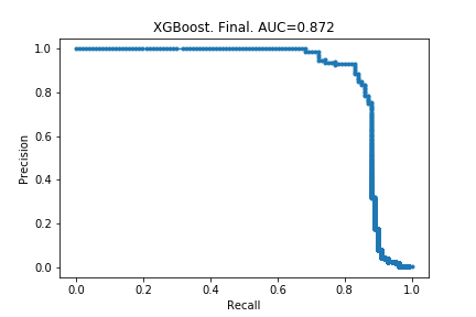
The optimal parameters changed (thankfully!). I then re-created the final model and this time there was an improvement:

Next time
My next blog post will be the final one in this series. I will summarise what I have done and what I have learnt. I will also have a look at what others did and see what I can learn from them.
The code
The code is provided for the Random Forest optimisation. The code for XGBoost is similar.
# import modules
import numpy as np
import pandas as pd

from sklearn.model_selection import train_test_split, KFold

from sklearn.metrics import precision_recall_curve
from sklearn.metrics import auc
from matplotlib import pyplot as plt
import seaborn as sns

from sklearn.ensemble import RandomForestClassifier
from xgboost import XGBClassifier

import itertools


#import data
data = pd.read_csv("creditcard.csv")
y = data.Class
X = data.drop(['Class', 'Time'], axis = 1)

#create train-valid versus test split
Xtv, X_test, ytv, y_test = train_test_split(X,y, random_state=0, test_size=0.2)


# create function which takes model and data
# returns auc

def auc_model(model, Xt, Xv, yt, yv):
    model.fit(Xt,yt)

    preds = model.predict_proba(Xv)
    preds = preds[:,1]

    precision, recall, _ = precision_recall_curve(yv, preds)
    auc_current = auc(recall, precision)

    return auc_current


# create options for hyperparameter
n_estimators = [40, 50, 60, 80]
max_depth = [None, 5, 10, 50]
max_features = ['auto', 3,5,7,10]
random_state = range(5)

# create frame to store auc data
auc_forest = pd.DataFrame({'n_estimators': [],
                           'max_depth': [],
                           'max_features': [],
                           'fold': [],
                           'auc': []
                          })


# loop through hyper parameter space

for n, md, mf, rs in itertools.product(n_estimators, max_depth, max_features, random_state):
    kf = KFold(n_splits = 4,
           shuffle = True,
           random_state = rs)

    model = RandomForestClassifier(n_estimators = n,
                                   max_depth = md,
                                   max_features = mf,
                                   random_state = 0)

    i=0
    for train, valid in kf.split(Xtv):
        Xt, Xv, yt, yv = Xtv.iloc[train], Xtv.iloc[valid], ytv.iloc[train], ytv.iloc[valid]

        # remove 99% of the non-fraudulent claims from training data to speed up fitting
        selection = (Xt.index % 100 == 1) | (yt == 1)
        Xt_reduced = Xt[selection]
        yt_reduced = yt[selection]

        auc_current = auc_model(model, Xt_reduced, Xv, yt_reduced, yv)
        auc_forest.loc[auc_forest.shape[0]] = [n, md, mf, 4*rs+i, auc_current]

        i+=1